Hydroelectric dam Model

Establishing and resolving a large optimization issue for profile optimization, constrained information fitted, parameter estimation, or other applications may be a challenging task. Thus, it's quite common to first setup and solve a smaller sized, easier form of the difficulty and then scale-up toward large-scale issue. Working with a smaller version reduces the time that it takes to identify key relationships in the model, makes the model easier to debug, and enables you to identify an efficient solution that can be used for the large-scale problem.

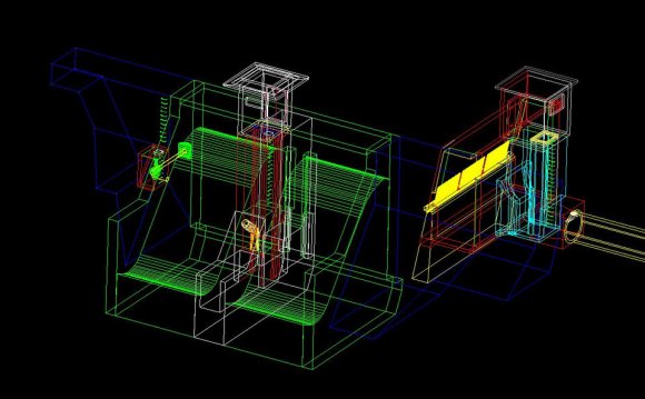
This article describes three approaches for finding a control strategy for optimal operation of a hydroelectric dam (Figure 1): utilizing a nonlinear optimization algorithm, a nonlinear optimization algorithm with derivative features, and quadratic programming.

Using the services of MATLAB®, Optimization Toolbox™ and Symbolic Math Toolbox™, we're going to begin by solving a smaller type of the situation then scale-up towards large-scale issue once we are finding an appropriate option technique.

Our hydroelectric power-plant model includes the inlet flow in to the reservoir from the lake and the storage amount of the reservoir (Figure 2).

Water-can leave the reservoir either through the spillway or through the turbine. Liquid that simply leaves through turbine is used to create electrical energy. We could offer this electrical energy at costs that are determined by different market factors. We control the rates from which water flows through spillway in addition to turbine. Our objective is to find values for those rates that'll maximize income over the long term.

The greatest values for the hydroelectric circulation rates are observed over a number of days at hourly intervals. As a result, we must discover the flow values at each and every hour, therefore how big the situation increase the longer we run the optimization.

Defining System Interactions Utilizing Symbolic Variables

We use the following equations to explain the communications inside system. The foremost is the empirical equation for turbine, and relates the electricity created into turbine movement and reservoir level. The 2nd provides the reservoir storage degree as a function associated with movement into and out of the reservoir.

Electricity(t) = TurbineFlow(t-1)*[½ k1(Storage(t) + Storage(t-1)) + k2]
Storage(t) = Storage(t-1) + ∆t * [inFlow(t-1) - spillFlow(t-1) - turbineFlow(t-1)]

The amount of electrical energy produced is a function of the quantity of water-flowing into the turbine while the storage space amount into the reservoir. Which means the larger the water level within the reservoir, the greater amount of energy are going to be produced for confirmed turbine circulation.

Specific limitations have to be taken into consideration. The reservoir degree and downstream movement rates must remain within certain ranges. The most standard of flow that turbine can handle is scheduled, however the spillway level is unrestricted. Also, the reservoir level at the conclusion of the simulation must be the same as the particular level in the beginning of the simulation. The energy plant will continue to operate beyond the time that we're optimizing, therefore we must avoid the solver from finding a remedy that empties the reservoir.

All the limitations for this issue tend to be linear, indicating they can be expressed in matrix notation. Our goal, however, is nonlinear, making it difficult to show. We start by formulating the objective purpose making use of symbolic variables.

X = sym('x', [2*N, 1]); percent turbine circulation and spill circulation
F = sym('F', [N, 1]); percent movement in to the reservoir
P = sym('P', [N, 1]); per cent price
s0 = sym('s0'); % preliminary storage
c = sym({'c1', 'c2', 'c3', 'c4'}.', 'r'); per cent constants

per cent Total out circulation equation
TotFlow = X(1:N)+X(N+1:end); per cent turbine flow + spill flow
% Storage Equations
S = cell(N, 1);
S{1} = s0 + c(1)*(F(1)-TotFlow(1));
for ii = 2:N
S{ii} = S{ii-1} + c(1)*(F(ii)-TotFlow(ii));
end
percent K aspect equation
k = c(2)*([s0; S(1:end-1)]+ S)/2+c(3);
per cent Megawatt-hours equation
MWh = k.*X(1:N)/c(4);
per cent Revenue equation
Roentgen = P.*MWh;
% complete income (Minus sign changes from maximization to minimization)
totR = -sum(R);

We convert this symbolic representation of your objective function into a MATLAB purpose with the matlabfunction demand.

We are able to today solve this problem using fmincon, an over-all nonlinear optimization solver.

percent Perform substitutions to make certain that X is the just continuing to be adjustable
totR = subs(totR, [c;s0;P;F], [C';stor0;price;inFlow]);
per cent Generate a MATLAB file from equation
matlabFunction(totR, 'vars', {X}, 'file', 'objFcn');
%% 5 - Optimize with FMINCON
options = optimset('MaxFunEvals', Inf, 'MaxIter', 5000...
'Algorithm', 'interior-point');
[x1, fval1] = fmincon(@objFcn, x0, A, b, Aeq, beq, LB, UB, , options);

Figure 3 reveals the optimization outcomes, with the electricity cost information that has been made use of.

We come across the ideal operation delivers no liquid to your spillway, and directs more water towards turbine when electricity costs increase.

Speeding Up Computations with Derivative Functions

The fmincon solver took 21.4 seconds to find the solution. Most of this time was invested approximating the gradient of this unbiased purpose utilizing finite distinctions. One method to increase this optimization issue is to provide the solver with features that analytically calculate its gradient and Hessian. Because we defined our objective function making use of symbolic math, we could make use of the gradient and hessian features from Symbolic mathematics Toolbox to determine these features immediately.

gradObj = gradient(totR, X); percent Gradient
matlabFunction(gradObj, 'vars', {X}, 'file', 'grad');
percent Create a purpose that returns the aim worth and gradient
ValAndGrad = @(x) deal(objFcn(x), grad(x));
hessObj = hessian(totR, X); percent Hessian
matlabFunction(hessObj, 'vars', {X}, 'file', 'Hess');
hfcn = @(x, lambda) Hess(x); % purpose handle to hessian
percent Optimize
options = optimset(options, 'GradObj', 'on', 'Hessian', 'user-supplied'...
'HessFcn', hfcn);
[x2, fval2] = fmincon(ValAndGrad, x0, A, b, Aeq, beq, LB, UB, , choices);

This time, the problem ended up being fixed in 0.25 moments. By specifying the gradient in addition to Hessian because of this problem, we obtained an 85-fold speedup.